排序多个链表

思路:

emmm… 采取上次的想法试试

一次只排序一个, 排序多次

代码:

1
2
3
4
5
6
7
8
9
10
11
12
13
14
15
16
17
18
19
20
21
22
23
24
25
26
27
28
29
30
31
32
33
34

class Solution {
public:
    ListNode* mergeKLists(vector<ListNode*>& lists) {
        ListNode *result = new ListNode(0);
        ListNode *backup = result;

        while (true) {
            int indexmin = 0;
            while(indexmin < lists.size() && !lists[indexmin])
                ++indexmin;

            ListNode *min = nullptr;
            if (indexmin < lists.size())
                min = lists[indexmin];
            else {
                if (indexmin > 0 && lists[indexmin - 1])
                    backup->next = lists[indexmin];
                break;
            }

            for (int i = 1; i < lists.size(); ++i)
                if (lists[i] && lists[i]->val < min->val) {
                    min = lists[i];
                    indexmin = i;
                }

            backup->next = min;
            backup = backup->next;
            lists[indexmin] = lists[indexmin]->next;
        }

        return result->next;
    }
};

一次循环内只思考得到最小的一个

代码的复杂度降低了, 码字速度和debug频率也明显好多了

结果

emmmmmm…. , 这是我至今为止做的最差的一次leetcode…

难的, 想不出好方法的. 即使有想法也不做. 所以平均来说一直还算中游

不过差不多意料之中, 毕竟 hard 还是没那么容易的(除了那次用标准库偷鸡, 虽然说偷完就后悔了)

那么, 要不要看一下dalao的代码?

算了吧, 这次没怎么仔细思考算法, 刚好想尝试一下降低循环复杂度

(虽然说尝试炸了, 但还算有所收获. 在时间紧迫, 还有其他适当因素的情况下, 这种做法可以说是最有效率的)

没怎么思考就去看别人的答案, 那我还做leetcode干嘛…

但是好像又暂时想不出什么好方法, 留到以后来优化吧…

给一个数组, 求其中三数和为零的所有组合, 要求不能重复

思路:

遍历数组, 找出所有三数集合, 再判断是否为零, 之后用一个map去重

代码:

1
2
3
4
5
6
7
8
9
10
11
12
13
14
15
16
17
18
19
20
21
22
23
24
25
26
27
28
29

class Solution {
public:
    vector<vector<int>> threeSum(vector<int>& nums) {
        if (nums.size() < 3) return {};

        vector<vector<int>> result;
        map<int, bool> repetitive;

        for (int i = 0; i < nums.size() - 2; ++i)
            for (int k = i + 1; k < nums.size() - 1; ++k)
                for (int v = k + 1; v < nums.size(); ++v) {
                    if (nums[i] + nums[k] + nums[v] != 0) continue;
                    else {
                        int nmax = max(nums[i], nums[k]);
                        nmax = max(nmax, nums[v]);
                        int nmin = min(nums[i], nums[k]);
                        nmin = min(nmin, nums[v]);

                        if (!repetitive[(nmax << 4) + nmin]) {
                            repetitive[(nmax << 4) + nmin] = true;
                            result.push_back({ nmin, 0 - nmin - nmax, nmax });
                        }
                        else continue;
                    }
                }

        return result;
    }
};

实际上map去重那里有漏洞, “精心准备”的数字有可能骗过它

结果:

超时了, 看到那密密麻麻的红字, 感觉有点不妙

实测算法在数组长度为200时已经有明显的停顿

算法复杂度大概是 差不多O(n3) 的样子, 所以随着长度的增加, 时间复杂度的增加是很恐怖的

200有明显停顿的话. 3000大概能算个痛

那么得优化算法了, 怎么优化呢? 暂时想不到…

优化的想法:

现在的算法在第一次循环的时候会将下标[0, 1]和后续所有的下标组合

第二次循环的时候会将下标[1, 2]和后续所有下标组合

这里明显有可以提升的空间, 因为两次里面1重叠了, 同理, 后续的组合都有重叠

在200长度的算法中, 大致会有 4000000 次循环, 而最后的结果只有 6 个组合

想要优化的话应该从这里入手, 如何在逻辑上筛除掉一些可能但和又不为零的组合

怎么删除? emmmm… 想不到

判断字符串是都按正确格式闭合

思路:

当一个字符被看到时, 预料与之对应的字符, 当该字符不是预料的字符, 有两种可能

1. 失败
2. 被包含, 例如 ({}), 当看到 ‘(‘ 时候, 我们想要的是 ‘)’. 但该语句是合法的

如果是第二种, 那么 ‘(‘ 要被保存起来, 这种数据结构非常适合用栈来做

代码:

1
2
3
4
5
6
7
8
9
10
11
12
13
14
15
16
17
18
19
20
21
22
23
24
25

class Solution {
public:
    bool isValid(string s) {
        if (!s.size()) return true;
        if (s.size() < 2) return false;

        map<char, char> lettermap{
            {'(', ')'},
            {'{', '}'},
            {'[', ']'},
        };
        vector<char> vch{ s[0] };
        for (int i = 1; i < s.size(); ++i) {
            if (lettermap[vch.back()] != s[i]) vch.push_back(s[i]);
            else {
                vch.pop_back();
                if (vch.size()) {}
                else if (++i < s.size())
                    vch.push_back(s[i]);
            }
        }

        return !vch.size();
    }
};

该代码并未在循环中判断是否合法

实际情况中, 可能一个非常长的字符串一开始就错了, 比如; “){}{}{}{}…”

但是依旧会将整个字符串循环一次, 这样做有三点考虑:

1. 代码更加简单, 简洁. 更容易理解
2. 如果代码的确需要很多判断才能确定结果, 那么多加条件语句反而是一种额外的消耗
   并且是O(n)复杂度, 节省的效率并不会有多少, 同时额外的消耗并不一定会比加条件语句多
3. 懒

PS: 如果能想到用栈结构来做这个题的话, 会方便很多. 如果没想到的话, 可能会越想越难.

Understanding Generated Columns

The Theory

Generated Columns is a feature released on MySQL 5.7. They can be used during CREATE TABLEor ALTER TABLE statements. It is a way of storing data without actually sending it through the INSERT or UPDATE clauses in SQL. The database resolves what the data will be.

生成列是在 MySQL 5.7 之后发布的一个特性, 可以在 CREATE TABLE / ALTER TABLE 期间使用. 是一种存储数据而不通过 INSERT / UPDATE 子句的方法. 数据库解析数据是什么

There are two types of Generated Columns: Virtual and Stored. They work with:

• mathematical expressions (product_price * quantity)
• built-in functions (RIGHT(), CONCAT(), FROM_UNIXTIME(), JSON_EXTRACT())
• literals (“2”, “new”, 0)

有两种生成列: virtual 和 stored, 它们工作于:

• 数学表达式
• 内建函数
• 复合常量

Besides that, they can be indexed but they don’t allow subqueries in it.
A Generated Column works within the table domain. If you need subqueries on a particular column, you may have to look at Views.

如上, 它们能够被索引, 但不允许子查询.

生成列在表域中工作, 如果你需要在特殊的列上子查询, 你需要考虑 view

The basic example

As an example I am going to use an e-commerce database as based on my past experience of what I have seen and worked. You will probably have at least these tables or something similar:

• users – stores user info
• products – stores product info like price and description
• orders – stores the user_id, date of order
• orders_items – stores product_id, order_id, quantity and price at the time of purchase

This is the whole DB: Gist.

Notice the order_items definition:

1
2
3
4
5
6
7
8
9
10

CREATE TABLE `orders_items` (
  `id` int(10) unsigned NOT NULL AUTO_INCREMENT,
  `order_id` int(10) unsigned NOT NULL,
  `product_id` int(10) unsigned NOT NULL,
  `product_price` decimal(10,2) unsigned NOT NULL DEFAULT '0.00',
  `quantity` int(10) unsigned NOT NULL DEFAULT 1,
  `created_at` timestamp NOT NULL DEFAULT CURRENT_TIMESTAMP,
  `updated_at` varchar(45) NOT NULL DEFAULT 'CURRENT_TIMESTAMP ON UPDATE CURRENT_TIMESTAMP',
  PRIMARY KEY (`id`)
) ENGINE=InnoDB AUTO_INCREMENT=1 DEFAULT CHARSET=utf8mb4;

The retrieval would bring:

1
2
3
4

SELECT
  `id`, `order_id`, `product_id`, `product_price`, `quantity`
FROM `orders_items`
LIMIT 5;

One example is to get the total of that order_item row, something like total_item_price that would store the value of product_price * quantity to show how much the summed amount of an item would be. Some databases have the MONEY type to store price, as with MySQL it is recommended to work with DECIMAL.

上述例子获取 order_item 所有行, 应该有类似 total_item_price 的列存储 product * quantity, 显示总额.

一些数据库有 MONEY 类型存储价格, MySQL 推荐使用 DECIMAL

People solve this problem in different ways:

• store the calculated price on a new column to make it easier to retrieve;
• create a view;
• or they calculate in the application itself, which in this case might cause problems due to how the language handles floats. There are libraries to deal with money values in a lot of languages and frameworks, however, the overhead of converting each row into a money object could be costly depending on the amount of data being transferred.

有几种不同的方式解决这个问题:

• 在新的列存储计算好的值, 便于检索
• 创建视图
• 或者在应用层计算, 由于不同语言对于浮点数的管理可能造成问题. 大量的语言和框架提供了库处理这个问题.然而, 将每行转换为对象的消耗依赖于有多少数据被调入

Another way I’ve seen is: people calculate in the query the total amount for the orders_items row as product_price * quantity:

还有一种我见过的方法 : 在查询中计算总额

1
2
3
4
5
6
7
8
9

SELECT
  `id`, 
  `order_id`, 
  `product_id`, 
  `product_price`, 
  `quantity`,
  `product_price` * `quantity` AS total_item_price
FROM `orders_items`
LIMIT 5;

Virtual Columns

• They take no disk space, except when using a Virtual Column as in a Secondary Index.
• They are an INPLACE operation: it means the table definition is changed without having to recopy all the data again. More info.
• The values are calculated on the fly during read operations and BEFORE triggers.

Consider using virtual columns for data where changes happens in a significant number of times. The cost of a Virtual Column comes from reading a table constantly and the server has to compute every time what that column value will be.

• 不占磁盘空间, 除非使用虚拟列作为次级索引
• 是 INPLACE 操作 : 这意味着表定义更改不需要拷贝所有数据
• 值在读取操作和 BEFORE 触发之间动态计算

Stored Columns

• They do use disk space.
• It has the same cost of adding a new column, so it is a COPY operation
• Values are updated in every INSERT and UPDATE statement.

You should consider using Stored Columns for when the data doesn’t change significantly or at all after creation, like for instance, the example above with the orders_items table. Once a purchase is made, the price of the product is stored, not being changed, neither the quantity. Considering this information we could create total_item_price as a Stored Column.

• 耗费磁盘空间
• 和增加行有相等的消耗, 等价于 COPY 操作
• 值在每次 INSERT 和 UPDATE 语句中更新

你需要考虑使用存储列, 以便数据没有显著变化或在创建后没有显著变化, 例如上面带有 order_items 的表. 当购买操作后, 存储产品的价格, 不会再更改, 数量也不会. 考虑到这个信息, 我们应该创建 total_item_price 存储列

The code

Creating a table

1

`-- Virtual Column` `CREATE` `TABLE` ``orders_items` (```id` ``int``(10) unsigned ``NOT` `NULL` `AUTO_INCREMENT,```order_id` ``int``(10) unsigned ``NOT` `NULL``,```product_id` ``int``(10) unsigned ``NOT` `NULL``,```product_price` ``decimal``(10,2) unsigned ``NOT` `NULL` `DEFAULT` `'0.00'``,```quantity` ``int``(10) unsigned ``NOT` `NULL` `DEFAULT` `1,```total_item_price` ``decimal``(10,2) ``AS` `(`quantity` * `product_price`),```created_at` ``timestamp` `NOT` `NULL` `DEFAULT` `CURRENT_TIMESTAMP``,```updated_at` ``varchar``(45) ``NOT` `NULL` `DEFAULT` `'CURRENT_TIMESTAMP ON UPDATE CURRENT_TIMESTAMP'``,``PRIMARY` `KEY` `(`id`)``) ENGINE=InnoDB AUTO_INCREMENT=1 ``DEFAULT` `CHARSET=utf8mb4;` `-- Stored Column` `CREATE` `TABLE` ``orders_items` (```id` ``int``(10) unsigned ``NOT` `NULL` `AUTO_INCREMENT,```order_id` ``int``(10) unsigned ``NOT` `NULL``,```product_id` ``int``(10) unsigned ``NOT` `NULL``,```product_price` ``decimal``(10,2) unsigned ``NOT` `NULL` `DEFAULT` `'0.00'``,```quantity` ``int``(10) unsigned ``NOT` `NULL` `DEFAULT` `1,```total_item_price` ``decimal``(10,2) ``AS` `(`quantity` * `product_price`) STORED,```created_at` ``timestamp` `NOT` `NULL` `DEFAULT` `CURRENT_TIMESTAMP``,```updated_at` ``varchar``(45) ``NOT` `NULL` `DEFAULT` `'CURRENT_TIMESTAMP ON UPDATE CURRENT_TIMESTAMP'``,``PRIMARY` `KEY` `(`id`)``) ENGINE=InnoDB AUTO_INCREMENT=1 ``DEFAULT` `CHARSET=utf8mb4;`

Notice how the definition changes on line 9 and 23: you have another keyword, AS, then an expression and specifically on line 23 you see a STORED keyword. In both lines they are generated columns, if nothing is specified will be a VIRTUAL column.

注意在 9 行 和 23 行的更改, 有另一个关键字, AS, 随之表达式和 STORED 关键字. 如果没有指定, 将会是一个 VIRTUAL 列

Altering a table

It uses the same syntax as adding a column, just adding the “AS (expression)” after the data type:

1

`-- `full_name` as VIRTUAL COLUMN``ALTER` `TABLE` `users``ADD` `COLUMN` ``full_name` ``VARCHAR``(500)``AS` `(CONCAT_WS(``" "``, `first_name`, `last_name`));` `-- `total_item_price` as STORED COLUMN``ALTER` `TABLE` `orders_items``ADD` `COLUMN` ``total_item_price` ``DECIMAL``(10, 2)``AS` `(`quantity` * `product_price`) STORED;`

JSON fields

It is also possible to extract data from JSON fields using generated columns. As the functions for JSON are built-in, JSON_EXTRACT and JSON_UNQUOTE as well “->” and “->>” work as expressionsfor a generated column:

1

`-- Stored Columns``ALTER` `TABLE` ``twitter_users```ADD` `COLUMN` ``location` ``VARCHAR``(255)``AS` `(response->>``"$.location"``) STORED;`

Final considerations

When the type is STORED, it must be specified after the expression otherwise the default behaviour will be to be VIRTUAL.

Generated columns can have indexes created as the following, no matter if stored, virtual or extracted from a JSON field:

1

`ALTER` `TABLE` `users``ADD` `INDEX` ``ix_full_name` (`full_name`);`

Which is the same syntax for normal columns.

brief

短变量声明

go可以使用形如 := 的方式定义变量, 这样的用法仅允许在函数内使用

( 同时, 在一个 := 的使用中可以定义, 也可以赋值, 不过我不建议也不会使用这样歧义的用法)

(同样的, := 支持变量的类型不同, 不过这也是比较歧义的用法, 不推荐)

指针

go的指针并没有什么不同. 为了安全性, 它抛弃了一些灵活性

它不支持指针运算, 相当于一个引用 ( 我不开心 :( )

new

1
2
3
4

i := 0
p := &i

p := new(i)

new 在 go 中的作用很小, 它的作用就相当于少了一个名字被占用

多重赋值

go 会先对右边的表达式一次性求值

生命周期

go 采用垃圾回收, 三色标记

slice

slice 相当于 vector, 但他必须依赖于另一个容器, 比如数组

可以挑战 slice 指向数组的那些区间, 同时可以动态增长

增长的区间一旦超过原容器的容量, 会在不更改原容器的情况下 重新分配并拷贝元素

json, xml…

go 提供了这些格式的转换支持

emmmm…, 感觉 go 使用起来很方便

安全的指针, 方便的变量命名, 垃圾回收, 多重赋值, 多返回值, for衍生while …

method

go 的方法声明和定义独立与对象本身

go 的方法就像一个指定了目标的函数

封装

go 以其不能随意命名为代价(这样的代价仅仅是不能随意首字母大小写)换来了简洁的封装规范

首字母大写的, 即为 public 成员, 而首字母小写的, 即为 private 成员. 这相当容易判断

@brief

when I learning java by , I see “The order of initialization is statics first…”. so… what about c++?

当我通过 thinking in java 学 java 时, 我注意到书中的一句话 “The order of initialization is statics first”. 那么, c++ 中是怎样对待的呢?

static

think this code:

1
2
3
4
5
6
7
8
9
10
11
12
13
14
15
16
17
18
19
20
21
22
23

class A{
public:
    int i2 = 1;
    static int i;
    A() { cout << "hello" << endl; }
};

int A::i = 10;

void f() {
    A a;
    cout << A::i << endl;
    A::i = 100;
}

int main() {
    A a;
    cout << A::i << endl;           
    thread t1(f);
    thread t2(f);
    t1.join();
    t2.join();
}

class A has a static field i, it’s an integer with default value 10.

how did these codes do?

类 A 有一个静态字段 i, 这是一个具有默认值为10的整型字段

assembly time

1
2
3
4
5
6
7
8
9
10
11
12
13
14
15
16
17
18
19
20
21
22
23
24
25
26
27
28
29
30
31
32
33
34
35
36
37
38
39
40
41
42
43
44
45
46
47
48
49
50
51
52
53
54
55
56
57
58
59
60
61
62

_ZN1A1iE:
▹   .long▹  10
▹   .text
▹   .globl▹ _Z1fv
▹   .type▹  _Z1fv, @function	
_Z1fv:
.LFB3324:
▹   .cfi_startproc
▹   pushq▹  %rbp
▹   .cfi_def_cfa_offset 16
▹   .cfi_offset 6, -16
▹   movq▹   %rsp, %rbp
▹   .cfi_def_cfa_register 6
▹   subq▹   $16, %rsp
▹   leaq▹   -4(%rbp), %rax
▹   movq▹   %rax, %rdi
▹   call▹   _ZN1AC1Ev
▹   movl▹   _ZN1A1iE(%rip), %eax // _ZN1A1iE
▹   movl▹   %eax, %esi
▹   leaq▹   _ZSt4cout(%rip), %rdi
▹   call▹   _ZNSolsEi@PLT
▹   movq▹   %rax, %rdx
▹   movq▹   _ZSt4endlIcSt11char_traitsIcEERSt13basic_ostreamIT_T0_ES6_@GOTPCREL(%rip), %rax
▹   movq▹   %rax, %rsi
▹   movq▹   %rdx, %rdi
▹   call▹   _ZNSolsEPFRSoS_E@PLT
▹   movl▹   $100, _ZN1A1iE(%rip)
▹   nop
▹   leave                                                                                  
▹   .cfi_def_cfa 7, 8
▹   ret
...
main:
.LFB3325:                                                                                 
▹   .cfi_startproc
▹   .cfi_personality 0x9b,DW.ref.__gxx_personality_v0
▹   .cfi_lsda 0x1b,.LLSDA3325
▹   pushq▹  %rbp
▹   .cfi_def_cfa_offset 16
▹   .cfi_offset 6, -16
▹   movq▹   %rsp, %rbp
▹   .cfi_def_cfa_register 6
▹   pushq▹  %rbx
▹   subq▹   $40, %rsp
▹   .cfi_offset 3, -24
▹   leaq▹   -20(%rbp), %rax
▹   movq▹   %rax, %rdi
.LEHB0:
▹   call▹   _ZN1AC1Ev
▹   movl▹   _ZN1A1iE(%rip), %eax // _ZN1A1iE
▹   movl▹   %eax, %esi
▹   leaq▹   _ZSt4cout(%rip), %rdi
▹   call▹   _ZNSolsEi@PLT
▹   movq▹   %rax, %rdx
▹   movq▹   _ZSt4endlIcSt11char_traitsIcEERSt13basic_ostreamIT_T0_ES6_@GOTPCREL(%rip), %rax
▹   movq▹   %rax, %rsi
▹   movq▹   %rdx, %rdi
▹   call▹   _ZNSolsEPFRSoS_E@PLT
▹   leaq▹   -32(%rbp), %rax
▹   leaq▹   _Z1fv(%rip), %rsi
▹   movq▹   %rax, %rdi
▹   call▹   _ZNSt6threadC1IRFvvEJEEEOT_DpOT0_

so, static value initialize while process run then copy to register while class construct function executed

所以, 静态变量随着程序运行而初始化, 随后在类构造函数完成后, 将其值拷贝到寄存器

this can also be discovered in gdb

1
2
3
4
5
6
7
8
9
10
11
12
13
14
15
16
17
18
19

(gdb) b main
Breakpoint 1 at 0x1908: file t.cpp, line 33.
(gdb) c
The program is not being run.
(gdb) r
Starting program: /root/cpp/a.out 
[Thread debugging using libthread_db enabled]
Using host libthread_db library "/lib/x86_64-linux-gnu/libthread_db.so.1".

Breakpoint 1, main () at t.cpp:33
33	    A a;
(gdb) p A::i
$2 = 10
(gdb) p &A::i
$3 = (int *) 0x555555758100 <A::i>
(gdb) p (int)0x555555758100
$4 = 1433764096
(gdb) p {int}0x555555758100
$5 = 10

how about static const?

1
2
3
4
5
6
7
8
9
10
11
12
13
14
15
16
17
18
19
20
21
22
23
24
25
26
27
28
29
30
31
32
33
34
35
36
37
38
39
40
41

class A{
public:
    int i2 = 1;
    static int const i = 11;
    A() { cout << "hello" << endl; }
};
...
_Z1fv:
.LFB3324:
▹   .cfi_startproc
▹   pushq▹  %rbp
▹   .cfi_def_cfa_offset 16
▹   .cfi_offset 6, -16
▹   movq▹   %rsp, %rbp 
▹   .cfi_def_cfa_register 6
▹   subq▹   $16, %rsp
▹   leaq▹   -4(%rbp), %rax
▹   movq▹   %rax, %rdi
▹   call▹   _ZN1AC1Ev
▹   movl▹   $11, %esi        // *       
▹   leaq▹   _ZSt4cout(%rip), %rdi
...
main:
.LFB3325:
▹   .cfi_startproc
▹   .cfi_personality 0x9b,DW.ref.__gxx_personality_v0
▹   .cfi_lsda 0x1b,.LLSDA3325
▹   pushq▹  %rbp
▹   .cfi_def_cfa_offset 16
▹   .cfi_offset 6, -16
▹   movq▹   %rsp, %rbp
▹   .cfi_def_cfa_register 6
▹   pushq▹  %rbx
▹   subq▹   $40, %rsp
▹   .cfi_offset 3, -24
▹   leaq▹   -20(%rbp), %rax
▹   movq▹   %rax, %rdi
.LEHB0:
▹   call▹   _ZN1AC1Ev
▹   movl▹   $11, %esi             // *                       
▹   leaq▹   _ZSt4cout(%rip), %rdi

if you use static const, there no space to store value, just a compile-time const value

如果使用static const, 则不会有空间存储值, 则是一个编译时常量

15.6.2.3 Sorted Index Builds

There are three phases to an index build. In the first phase, the clustered index is scanned, and index entries are generated and added to the sort buffer. When the sort buffer becomes full, entries are sorted and written out to a temporary intermediate file. This process is also known as a “run”. In the second phase, with one or more runs written to the temporary intermediate file, a merge sort is performed on all entries in the file. In the third and final phase, the sorted entries are inserted into the B-tree.

索引构建有三个阶段, 第一阶段, 扫描聚簇索引, 生成索引条目, 添加到排序缓存中. 当排序缓存被填满时, 条目数据排序并存储到临时的中间文件. 这个过程也被成为 ‘run’, 第二阶段, 随着 ‘runs’ 写入到临时中间文件, 对所有文件中的条目数据执行合并排序, 第三阶段, 排序好的条目数据插入到 B-tree 中.

Prior to the introduction of sorted index builds, index entries were inserted into the B-tree one record at a time using insert APIs. This method involved opening a B-treecursor to find the insert position and then inserting entries into a B-tree page using an optimistic insert. If an insert failed due to a page being full, a pessimistic insert would be performed, which involves opening a B-tree cursor and splitting and merging B-tree nodes as necessary to find space for the entry. The drawbacks of this “top-down”method of building an index are the cost of searching for an insert position and the constant splitting and merging of B-tree nodes.

在引进有序索引构建之前, 使用插入 APIs 一次一条, 将索引条目插入到 B-tree 中. 这个方法包括打开 B-tree 光标, 查找插入位置, 然后使用 optimistic 插入数据到 B-tree 页中.

如果因为页面已满而插入失败, 执行 pessimistic 插入, 包括打开 B-tree 光标, 并根据需要分裂合并 B-tree 节点, 以便为条目找到空间.

Sorted index builds use a “bottom-up” approach to building an index. With this approach, a reference to the right-most leaf page is held at all levels of the B-tree. The right-most leaf page at the necessary B-tree depth is allocated and entries are inserted according to their sorted order. Once a leaf page is full, a node pointer is appended to the parent page and a sibling leaf page is allocated for the next insert. This process continues until all entries are inserted, which may result in inserts up to the root level. When a sibling page is allocated, the reference to the previously pinned leaf page is released, and the newly allocated leaf page becomes the right-most leaf page and new default insert location.

有序索引使用自底向上方法构建索引, 使用这种方法, 所有 B-tree 层级都有一个指向最右叶子页的引用. 最右叶子页在必要的 B-tree 深度分配, 条目根据他们有序顺序插入. 当叶子节点满了, 父节点增加一个节点指针, 为下一次插入分配一个 sibling 叶子页. 这个过程持续到所有的条目插入为止, 可能导致插入到根层级.

当 sibling 页分配后, 指向之前固定的叶子页的引用被释放, 新分配的叶子页成为最右叶子页和新的插入位置

(PS. 和自平衡二叉树类似, 插入节点到尾端节点, 不断上溢到适当的位置)

Reserving B-tree Page Space for Future Index Growth

To set aside space for future index growth, you can use the innodb_fill_factor configuration option to reserve a percentage of B-tree page space. For example, setting innodb_fill_factor to 80 reserves 20 percent of the space in B-tree pages during a sorted index build. This setting applies to both B-tree leaf and non-leaf pages. It does not apply to external pages used for TEXT or BLOB entries. The amount of space that is reserved may not be exactly as configured, as the innodb_fill_factor value is interpreted as a hint rather than a hard limit.

为了设置空间为以后的索引增长做准备, 可以使用 innodb_fill_factor 设置存储百分比 B-tree 页空间, 比如, 设置 innodb_fill_factor 为 80, 存储 20% 的空间. 这个设置引用于所有 B-tree 叶和非叶页, 不适用于 TEXT / BLOB 条目的页.

存储的页面大小不一定精准, innodb_fill_factor 是一个提示, 而并不是硬限制

Sorted Index Builds and Full-Text Index Support

Sorted index builds are supported for fulltext indexes. Previously, SQL was used to insert entries into a fulltext index.

有序索引构建支持 fulltext index.

Sorted Index Builds and Compressed Tables

For compressed tables, the previous index creation method appended entries to both compressed and uncompressed pages. When the modification log (representing free space on the compressed page) became full, the compressed page would be recompressed. If compression failed due to a lack of space, the page would be split. With sorted index builds, entries are only appended to uncompressed pages. When an uncompressed page becomes full, it is compressed. Adaptive padding is used to ensure that compression succeeds in most cases, but if compression fails, the page is split and compression is attempted again. This process continues until compression is successful. For more information about compression of B-Tree pages, see Section 15.9.1.5, “How Compression Works for InnoDB Tables”.

对压缩表, 之前创建索引的方法将条目添加到压缩/未压缩页面, 当更改日志逐渐增多, 压缩页需要重压缩. 如果因为空间不足而压缩失败, 也需要被分割, 在有序构建中, 条目仅仅添加到未压缩页. 当未压缩页逐渐填满, 压缩该页.

在大多数情况下适应的填充用作确保压缩成功, 如果压缩失败, 页被分隔, 然后再次尝试压缩. 这个过程直到压缩成功为止.

Sorted Index Builds and Redo Logging

Redo logging is disabled during a sorted index build. Instead, there is a checkpoint to ensure that the index build can withstand a crash or failure. The checkpoint forces a write of all dirty pages to disk. During a sorted index build, the page cleaner thread is signaled periodically to flush dirty pages to ensure that the checkpoint operation can be processed quickly. Normally, the page cleaner thread flushes dirty pages when the number of clean pages falls below a set threshold. For sorted index builds, dirty pages are flushed promptly to reduce checkpoint overhead and to parallelize I/O and CPU activity.

在有序索引构建期间, redo logging 不可用. 代替其的是 checkpoint, 它确保索引构建禁得住错误和崩溃. checkpoint 强制脏页写回缓存.

Sorted Index Builds and Optimizer Statistics

Sorted index builds may result in optimizer statistics that differ from those generated by the previous method of index creation. The difference in statistics, which is not expected to affect workload performance, is due to the different algorithm used to populate the index.

this is a follow-up to sort

these sort algorithms based on <Algorithms, 4th>

shell sort

shell sort is a better version sort algorithm based on insert sort.

when a[0] is the biggest number but head of array, for move the number to the end of the array, need swap length(a) elements.

shell sort 是基于插入排序的改良版本

当 a[0] 是整个数组最大的元素时, 为了移动这个元素到数组的尾端, 需要交换 length(a) 次元素.

1
2
3
4
5
6
7
8
9
10
11

void shellSort(vector<int> &v) {
    int h = 0;
    while (h < v.size() / 3) h = h * 3 + 1;
    while (h >= 1) {
        for (int j = h; j < v.size(); ++j) {
            for (int i = j; i >= h && v[i] < v[i - h]; i -= h)
                swap(v[i], v[i - h]);                         
        }
        h /= 3;
    }
}

bottom-up sort

bottom-up sort is a down-top method based on merge sort.

bottom-up sort 基于合并排序, 是一种从底至上的方法

1
2
3
4
5
6
7
8
9
10
11
12
13
14
15
16
17
18
19
20
21

void merge(vector<int> &v, int b, int m, int e) {
    vector<int> v2 = v;
    int mid = m++;
    for (int i = b; i <= e; ++i) {
        if (b > mid)
            v[i] = v2[m++];
        else if (m > e)
            v[i] = v2[b++];
        else if (v2[b] < v2[m])
            v[i] = v2[b++];
        else·
            v[i] = v2[m++];
    }
}

void bottomupSort(vector<int> &v) {
	for (int i = 1; i < v.size(); i *= 2){
		for (int j = 0; j < v.size() - i; j = j + 2 * i)
			merge(v, j, j + i -1, min(int(v.size() - 1, j + 2 * i - 1)));
	}
}

a better version of quick sort

if an array with some duplicate numbers, skip these numbers will be more effective

1
2
3
4
5
6
7
8
9
10
11
12
13
14
15
16
17
18
19
20
21
22
23
24
25
26
27
28
29
30
31
32
33

#define QS_MIN_LENGTH 7

void quickSort(vector<int> &nums, int b, int e) {
    if (b >= e) return;                          

    // if element too little, insertSort more effective than quickSort
    if (e - b < QS_MIN_LENGTH)
        insertSort(nums, b, e);

    // meduim of three can get more effetive pivot
    int m = (b + e) / 2;
    if (nums[b] > nums[m])
        swap(nums[b], nums[m]);
    if (nums[b] > nums[e])
        swap(nums[b], nums[e]);
    if (nums[m] > nums[e])
        swap(nums[m], nums[e]);

    int pivot = nums[m];
    // skip elements equal pivot
    int lt = b + 1, eq = lt, gt = e - 1;
    while (eq <= gt) { 
        if (nums[eq] < pivot)
            swap(nums[lt++], nums[eq++]);
        else if (nums[eq] > pivot)
            swap(nums[eq], nums[gt--]);
        else
            eq++;
    }       

    quickSort(nums, b, lt - 1);
    quickSort(nums, gt + 1, e);
}

a sort algorithm without compare

I saw a string sort algorithm without compare in <algorithm 4th>. so take some notes

I’m to lazy to write this code, please check the book…

source link

Sort

Bubble Sort

Bubble is the most common algorithm to sort an array. It based on the idea of repeatedly comparing adjacent element and then swapping their value if exist in the wrong order

1
2
3
4
5
6
7
8

void bubbleSort(vector<int> &nums) {
    for (int i = 0; i < nums.size(); ++i) {
        for (int j = i + 1; j < nums.size(); ++j) {
            if (nums[i] > nums[j])
                swap(nums[i], nums[j]);
        }
    }
}

Selection sort

The selection sort is based on finding the minimum or maximum in an unsorted array and putting it to a sorted array

1
2
3
4
5
6
7
8
9
10

void selectionSort(vector<int> &nums) {
    for (int i = 0; i < nums.size(); ++i) {
        int min = i;
        for (int j = i + 1; j < nums.size(); ++j) {
            if (nums[min] > nums[j])
                min = j;
        }
        swap(nums[i], nums[min]);
    }
}

Insertion sort

From left to right, find each element’s correct position

1
2
3
4
5
6
7
8
9
10
11
12
13

void insertSort(vector<int> &nums) {
    for (int i = 1; i < nums.size(); ++i) {
        int v = nums[i];
        int j = i;
        while(j > 0) {
            nums[j] = nums[j - 1];
            if (nums[j] <= v)
                break;
            --j;                            
        }
        nums[j] = v;
    }
}

Merge sort

Merge sort is a divide-and-conquer algorithm based on repeatedly breaking down an array to two sub-array and then merge them

1
2
3
4
5
6
7
8
9
10
11
12
13
14
15
16
17
18
19
20
21
22
23
24
25
26

void merge(vector<int> &nums, int b, int e) {
    int m = (b + e) / 2;
    int q = m + 1, p = b;
    vector<int> v;
    for (int i = b; i <= e; ++i) {
        if (p > m)
            v.push_back(nums[q++]);
        else if (q > e)
            v.push_back(nums[p++]);
        else if (nums[q] > nums[p])
            v.push_back(nums[p++]);
        else
            v.push_back(nums[q++]);              
    }

    for (auto val : v)
        nums[b++] = val;
}

void mergeSort(vector<int> &nums, int b, int e) {
    if (b >= e) return;

    mergeSort(nums, b, (e + b) / 2);
    mergeSort(nums, (e + b) / 2 + 1, e);
    merge(nums, b, e);
}

Quick sort

Quick sort is also a divide-and-conquer algorithm. But it reduces the space complexity and removes the use of auxiliary array that is used in merger sort
One of the most important factors to influence performance is the pivot.
I chose the pivot from the middle, front, and back of the array. Sometimes will improve performance

1
2
3
4
5
6
7
8
9
10
11
12
13
14
15
16
17
18
19
20
21
22
23
24
25
26
27
28
29
30
31
32
33

int partion(vector<int> &nums, int b, int e) {
    int p = e;
    int m = (b + e) / 2;
    if (nums[b] > nums[m])
        swap(nums[b], nums[m]);
    if (nums[b] > nums[e])
        swap(nums[b], nums[e]);
    if (nums[m] > nums[e])
        swap(nums[m], nums[e]);

    int piv = nums[m];
    swap(nums[e--], nums[m]);
    while (b < e) {
        while (b < e && nums[b] < piv)
            ++b;
        while (b < e && nums[e] >= piv)
            --e;
        if (b >= e) break;

        swap(nums[b], nums[e]);
    }
    swap(nums[p], nums[b]);

    return b;
}

void quickSort(vector<int> &nums, int b, int e) {
    if (b >= e) return;

    int p = partion(nums, b, e);
    quickSort(nums, b, p - 1);
    quickSort(nums, p + 1, e);
}

Heap sort

Heap sort uses a structure called heap to sort the array. Heap is a complete binary tree.
left sub-tree index = 2 * root index + 1
right sub-tree index = 2 * root index + 2

1
2
3
4
5
6
7
8
9
10
11
12
13
14
15
16
17
18
19
20
21
22
23
24
25
26

void heapify(vector<int> &nums, int n, int i) {
    int largest = i;
    int l = 2 * i + 1;
    int r = l + 1;

    if (l < n && nums[l] > nums[largest])
        largest = l;

    if (r < n && nums[r] > nums[largest])
        largest = r;

    if (largest != i) {
        swap(nums[i], nums[largest]);
        heapify(nums, n, largest);
    }
}

void heapSort(vector<int> &nums) {                
    for (int i = nums.size() / 2 - 1; i >= 0; --i)
        heapify(nums, nums.size(), i);

    for (int i = nums.size() - 1; i >= 0; --i) {
        swap(nums[0], nums[i]);
        heapify(nums, i, 0);
    }
}

@brief

​ 早上地铁充值时有位大妈有东西掉了, 和工作人员沟通了几分钟, 本来就睡晚了, 最后差点导致上班迟到 = =

​ 然后突然想到这就是单线程啊… 于是就有了这篇关于 scheduler algorithm 的笔记

​ 原文

what is scheduler

Schedulers are special system software which handle process scheduling in various ways. Their main task is to select the jobs to be submitted into the system and to decide which process to run. There are three types of Scheduler:

schedulers 是特殊的系统软件, 通过多种方式控制进程调度. 它们主要的任务是选择任务并提交到系统, 决定哪个进程执行, 这里有三种类型的 scheduler

1. Long term (job) scheduler – Due to the smaller size of main memory initially all program are stored in secondary memory. When they are stored or loaded in the main memory they are called process. This is the decision of long term scheduler that how many processes will stay in the ready queue. Hence, in simple words, long term scheduler decides the degree of multi-programming of system.

   因为主存空间较小, 最初, 所有的程序都存储在次级内存, 当它们排序或加载到主存时, 称其为进程. 这取决于 long term scheduler , 它决定有多少进程保留在你准备队列中, 因此, 简单来说, long term scheduler 决定了系统的多程序程度

   (PS: 这里指的应该是内存和硬盘, 关于 secondary memory, 可以参考 secondary memory)

2. Medium term scheduler – Most often, a running process needs I/O operation which doesn’t requires CPU. Hence during the execution of a process when a I/O operation is required then the operating system sends that process from running queue to blocked queue. When a process completes its I/O operation then it should again be shifted to ready queue. ALL these decisions are taken by the medium-term scheduler. Medium-term scheduling is a part of swapping.

   运行中的进程经常需要 I/O 操作而并非 CPU. 因此在进程执行期间, 当需要 I/O 操作时, 操作系统将当前进程从运行中队列发送到阻塞队列. 当进程完成它的 I/O 操作时, 应该再次将它移回准备队列. 所有这些操作都由 medium-term scheduler 决定, medium-term scheduling 是 swapping 的一部分

3. Short term (CPU) scheduler – When there are lots of processes in main memory initially all are present in the ready queue. Among all of the process, a single process is to be selected for execution. This decision is handled by short term scheduler.Let’s have a look at the figure given below. It may make a more clear view for you.

   当由大量的进程在准备队列时, 在所有的进程中, 只有一个进程被选择执行. 这由 short term scheduler 决定.

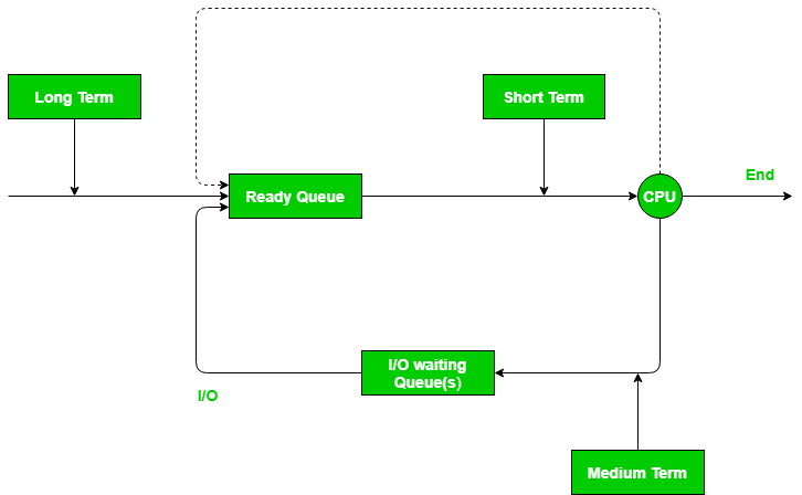
(PS: 关于 CPU burst time, determine burst time)

difference scheduling algorithms

First Come First Serve (FCFS): Simplest scheduling algorithm that schedules according to arrival times of processes. First come first serve scheduling algorithm states that the process that requests the CPU first is allocated the CPU first. It is implemented by using the FIFO queue. When a process enters the ready queue, its PCB is linked onto the tail of the queue. When the CPU is free, it is allocated to the process at the head of the queue. The running process is then removed from the queue. FCFS is a non-preemptive scheduling algorithm.

最简单的调度算法根据时间进程的时间顺序调度. 先到先得调度算法声明最先请求 CPU 的进程最先被处理. 其使用 FIFO 队列实现. 当进程进入准备队列时, PCB 链接到队列的尾部(??? 啥东西???) 当 CPU 空闲时, CPU 资源被分配给队列头部的进程. 运行中进程从队列中移除, FCFS 是一个非抢先式的调度算法

Note:First come first serve suffers from convoy effect.

FCFS 受 convoy effect 影响

Shortest Job First (SJF): Process which have the shortest burst time are scheduled first.If two processes have the same bust time then FCFS is used to break the tie. It is a non-preemptive scheduling algorithm.

拥有最短突发时间的进程优先调度. 当两个进程拥有同样的突发时间时, FCFS 用于解决这种情况. 它同样是一个非抢占调度算法

Longest Job First (LJF): It is similar to SJF scheduling algorithm. But, in this scheduling algorithm, we give priority to the process having the longest burst time. This is non-preemptive in nature i.e., when any process starts executing, can’t be interrupted before complete execution.

类似 SJF 调度算法, 但是, 在这个调度算法中, 给予最长突发时间优先权限. 这同样也是非抢占式的. 当进程开始执行时, 不能在完成执行前被打断

Shortest Remaining Time First (SRTF): It is preemptive mode of SJF algorithm in which jobs are schedule according to shortest remaining time.

是 SJF 调度算法的抢占版本, 根据最少剩余时间调度

Longest Remaining Time First (LRTF): It is preemptive mode of LJF algorithm in which we give priority to the process having largest burst time remaining.

LJF 算法的抢占模式, 给予最大突发时间剩余进程优先权限

Round Robin Scheduling: Each process is assigned a fixed time(Time Quantum/Time Slice) in cyclic way.It is designed especially for the time-sharing system. The ready queue is treated as a circular queue. The CPU scheduler goes around the ready queue, allocating the CPU to each process for a time interval of up to 1-time quantum. To implement Round Robin scheduling, we keep the ready queue as a FIFO queue of processes. New processes are added to the tail of the ready queue. The CPU scheduler picks the first process from the ready queue, sets a timer to interrupt after 1-time quantum, and dispatches the process. One of two things will then happen. The process may have a CPU burst of less than 1-time quantum. In this case, the process itself will release the CPU voluntarily. The scheduler will then proceed to the next process in the ready queue. Otherwise, if the CPU burst of the currently running process is longer than 1-time quantum, the timer will go off and will cause an interrupt to the operating system. A context switch will be executed, and the process will be put at the tail of the ready queue. The CPU scheduler will then select the next process in the ready queue.

每个进程每个周期被分配一个固定的时间(时间量子/时间片), 这特别为时间共享系统所设计. 准备队列被视作一个循环的队列. CPU 调度循环准备队列. 分配 CPU 资源给每个进程最多一个的时间量.

为了实现 round robin scheduling 将准备队列依旧保持为 FIFO 队列, 新的进程在队列的尾端加入, CPU 从队列的头部选取一个进程, 设置在一个时间量后中断的定时器, 派发这个进程. 这个进程的 CPU 突发可能少于1个时间量, 在这种情况下, 进程会自动释放 CPU 资源, 调度器继续处理准备队列的下一个进程, 其他情况下, 如果当前进程 CPU burst 超过1个时间片, 将会触发定时器, 向操作系统发出一个中断. 将会执行内容切换, 进程将会重新放入准备队列的尾端. CPU 调度将会选择准备队列的下一个进程, 以此循环.

Priority Based scheduling (Non-Preemptive): In this scheduling, processes are scheduled according to their priorities, i.e., highest priority process is scheduled first. If priorities of two processes match, then schedule according to arrival time. Here starvation of process is possible.

在这个调度下, 进程根据他们的优先级调度, 比如, 高优先级的进程会有限调度. 如果两个进程的优先级相等. 则根据他们的先后顺序调度, 有可能出现饥饿线程

Highest Response Ratio Next (HRRN): In this scheduling, processes with highest response ratio is scheduled. This algorithm avoids starvation.

Response Ratio = (Waiting Time + Burst time) / Burst time

在这种调度下, 拥有高响应比的进程有限调度, 这个算法避免饥饿

Multilevel Queue Scheduling: According to the priority of process, processes are placed in the different queues. Generally high priority process are placed in the top level queue. Only after completion of processes from top level queue, lower level queued processes are scheduled. It can suffer from starvation.

根据进程的优先级, 进程被放置在不同的队列. 通常, 高优先级的进程被放置在上层队列. 只有在完成上层队列中的进程后, 低层队列中的进程才会被调度, 它有可能挨饿

Multi level Feedback Queue Scheduling: It allows the process to move in between queues. The idea is to separate processes according to the characteristics of their CPU bursts. If a process uses too much CPU time, it is moved to a lower-priority queue.

允许进程在队列中移动, 这个想法根据它们的 CPU 突发特性区分进程, 如果进程使用过多的 CPU 时间, 它将会被移动到低优先级的队列

Some useful facts about Scheduling Algorithms:

1. FCFS can cause long waiting times, especially when the first job takes too much CPU time.

   FCFS 可能导致长时间等待, 特别是当第一个任务执行太久时

2. Both SJF and Shortest Remaining time first algorithms may cause starvation. Consider a situation when the long process is there in the ready queue and shorter processes keep coming.

   SJF 和 shortest remaining time first 算法可能导致饥饿, 考虑当长的进程在准备队列中, 但一直有短进程不断加入的情景

3. If time quantum for Round Robin scheduling is very large, then it behaves same as FCFS scheduling.

   如果 round robin 调度的时间量太长时, 情况类似于 FCFS 调度

4. SJF is optimal in terms of average waiting time for a given set of processes,i.e., average waiting time is minimum with this scheduling, but problems are, how to know/predict the time of next job.

   就给定一组进程的平均等待时间而言, SJF 是最优的, 但是问题在于, 如何预测下一个任务的执行时间